Kernel Trick I - Deep Convolutional Representations in RKHS
Convolutional Kernel Networks
Goal 🚀
Fear not, those who delved into the maths of the kernel trick, for its advent in deep learning is coming.
In this blog post, we focus on the Convolutional Kernel Network (CKN) architecture proposed in End-to-End Kernel Learning with Supervised Convolutional Kernel Networks
Kernel Trick 🧙♂️
Before diving into the CKN itself, we briefly recall what the kernel trick stands for. In many situations, one needs to measure the similarity between inputs. Such inputs would typically be mapped to a high-dimensional space and compared by computing their inner product. More formally, place yourself in your favorite high-dimensional feature space \(\mathcal{H}\) and consider a mapping \(\varphi\colon \mathcal{X} \to \mathcal{H}\). The similarity between two inputs \(\mathbf{x}, \mathbf{x}'\) the inner product \(\langle \varphi(\mathbf{x}), \varphi(\mathbf{x}')\rangle_{\mathcal{H}}\). The kernel trick enables us to avoid working with high-dimensional vectors in \(\mathcal{H}\) and directly evaluate such pairwise comparison by kernel evaluation, i.e.,
\[\begin{equation*} K(\mathbf{x}, \mathbf{x}') = \langle \varphi(\mathbf{x}), \varphi(\mathbf{x}')\rangle_{\mathcal{H}} \end{equation*}\]The kernel trick presents many advantages. One of whom is that, in practice, one can choose a kernel \(K\) such that the equation above holds for some map \(\varphi\), without needing to obtain \(\varphi\) in closed form. The existence of such kernels has been established in the rich literature on kernel methods. For the interested reader, more details can be found in
Positive definite kernels 
One of the most prominent examples of kernels for which the kernel trick can be applied is the class of positive definite (p.d.) kernels. Formally, a p.d. kernel is a function \(K : \mathcal{X}\times\mathcal{X} \to \mathbb{R}\) that is symmetric, i.e.,
\[\forall \mathbf{x},\mathbf{x}', ~K(\mathbf{x},\mathbf{x}') = K(\mathbf{x}',\mathbf{x}),\]and verifies
\[\forall (\mathbf{x}_1, \dots, \mathbf{x}_N) \in \mathcal{X}^N, (\alpha_1, \dots, \alpha_N) \in \mathbb{R}^N, \sum_{i=1}^N\sum_{j=1}^N \alpha_i \alpha_j K(\mathbf{x}_i,\mathbf{x}_j) \geq 0.\]In practice, assuming one wants to work with vectors of \(\mathbb{R}^d\), a p.d. kernel can be easily obtained by considering a mapping \(\varphi \colon \mathcal{X} \to \mathbb{R}^d\) and defining \(K \colon \mathcal{X}^2 \to \mathbb{R}\) as
\[\begin{equation*} K(\mathbf{x}, \mathbf{x}') = \langle \varphi(\mathbf{x}), \varphi(\mathbf{x}')\rangle_{\mathcal{H}}. \end{equation*}\]Surprisingly, the converse is also true, i.e., any p.d. kernel can be expressed as an inner product. More formally, the Aronszajn Theorem
One of the most direct and popular applications of the kernel trick is with Support Vector Machines (SVMs) where similarities are measured by a dot product in a high-dimensional feature space. Using the kernel trick makes the classification task easier and only requires kernel pairwise evaluation instead of explicitly manipulating high-dimensional vectors. The short animation below shows how the kernel trick can be used to map tangled data originally lying on a 2D plane to a higher dimensional space where they can be separated by a hyperplane.
It goes without saying that the range of applications of the kernel trick is large and goes beyond SVMs and making data linearly separable. In the rest of this post, we study how the kernel trick can be used to derive a new type of convolutional neural network that couples data representation and prediction tasks.
Convolutional Kernel Network in-depth 🔎
Now that everyone has a clear head regarding the kernel trick, we are prepared to introduce the so-called Convolutional Kernel Network. The main idea behind the CKN is to leverage the kernel trick to represent local neighborhoods of images. In this section, we explain how the authors build Convolutional Kernel layers that can be stacked into a multi-layer CKN.
Motivation: representing local image neighborhoods
The CKN architecture is a type of convolutional neural network that couples the prediction task with representation learning. The main novelty is to benefit from the kernel trick to learn nonlinear representations of local image patches. Formally, taking into account the $3$ color channels, an image can be described as a mapping \(I_0 \colon \Omega_0 \to \mathbb{R}^{3}\) where \(\Omega_0 \subset [0,1]^2\) is a set of pixel coordinates. Reusing the notations previously introduced, we can consider a p.d. kernel \(K\colon \mathcal{X} \times \mathcal{X} \to \mathbb{R}\) that is implicitly associated to a Hilbert space \(\mathcal{H}\), called the Reproducing Kernel Hilbert Space (RKHS), and a mapping \(\varphi \colon \mathcal{X} \to \mathcal{H}\). Considering two patches \(\mathbf{x}\) and \(\mathbf{x}'\) extracted from \(I_0\), their representation in \(\mathcal{H}\) is simply given by \(\varphi(\mathbf{x})\) and \(\varphi(\mathbf{x}')\). By definition, this embedding verifies
\[\begin{equation*} K(\mathbf{x}, \mathbf{x}') = \langle \varphi(\mathbf{x}), \varphi(\mathbf{x}')\rangle_{\mathcal{H}} \end{equation*}.\]The original CKN paper
The function \(\kappa(\langle \cdot, \cdot \rangle)\) should be a smooth dot-product kernel on the sphere whose Taylor expansion has non-negative coefficients to ensure positive definiteness. A common example of such dot-product kernel is the exponential kernel that verifies for inputs \(\mathbf{y}, \mathbf{y}'\) with unit \(\ell_2\) norm
\[\begin{equation*} \kappa_{\exp}(\mathbf{y},\mathbf{y}') = \text{e}^{\beta(\langle \mathbf{y},\mathbf{y}'\rangle -1)} = \text{e}^{-\frac{\beta}{2}\lVert \mathbf{y}-\mathbf{y}' \rVert_2^2} \end{equation*},\]for \(\beta > 0\). Taking \(\displaystyle\beta = \frac{1}{\sigma^2}\) leads to the well-known Gaussian (RBF) Kernel. We will see below that the parameter \(\beta\) can be learned along the training of the neural network.
From theory to practice
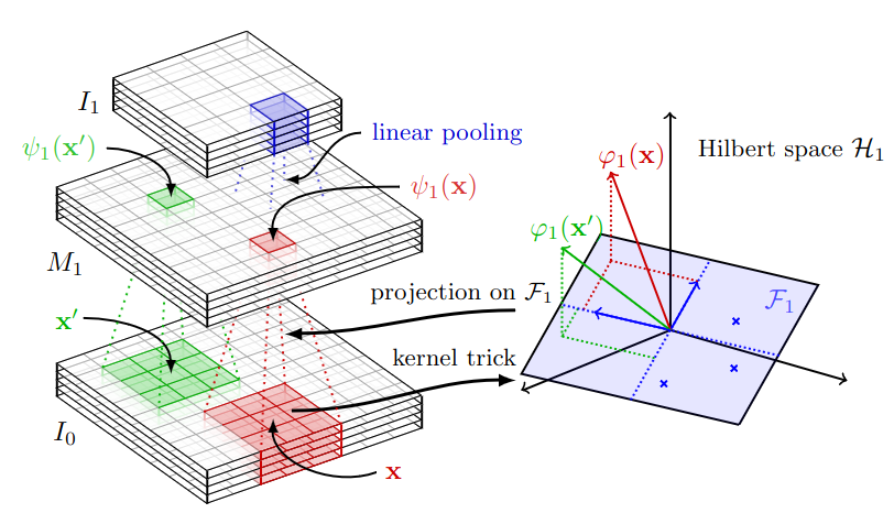
While the kernel trick is elegant and appealing from a mathematical perspective, one can wonder how to implement it in practice. Indeed, the RKHS \(\mathcal{H}\) can be of infinite dimension which makes it computationally intractable ![]() ! Fortunately, our friend Nyström comes to the rescue to approximate the feature representations \(\varphi(\mathbf{x})\) and \(\varphi(\mathbf{x}')\) by their projection \(\psi(\mathbf{x})\) and \(\psi(\mathbf{x}')\) onto a finite dimensional subspace \(\mathcal{F}\) (see the figure below).
! Fortunately, our friend Nyström comes to the rescue to approximate the feature representations \(\varphi(\mathbf{x})\) and \(\varphi(\mathbf{x}')\) by their projection \(\psi(\mathbf{x})\) and \(\psi(\mathbf{x}')\) onto a finite dimensional subspace \(\mathcal{F}\) (see the figure below).
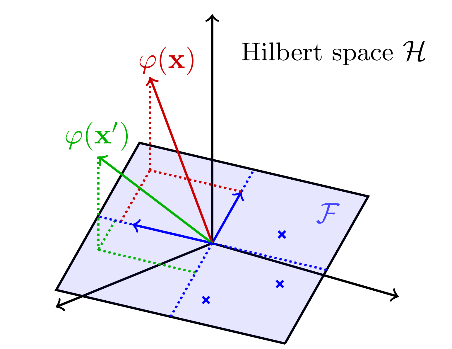
The subspace \(\mathcal{F}\) is defined as \(\mathcal{F} = \text{span}(z_1,\dots,z_p)\), where the \((z_i)_{i\in\{1\dots p\}}\) are anchor points of unit-norm. As explained in
Building a Convolutional Kernel layer
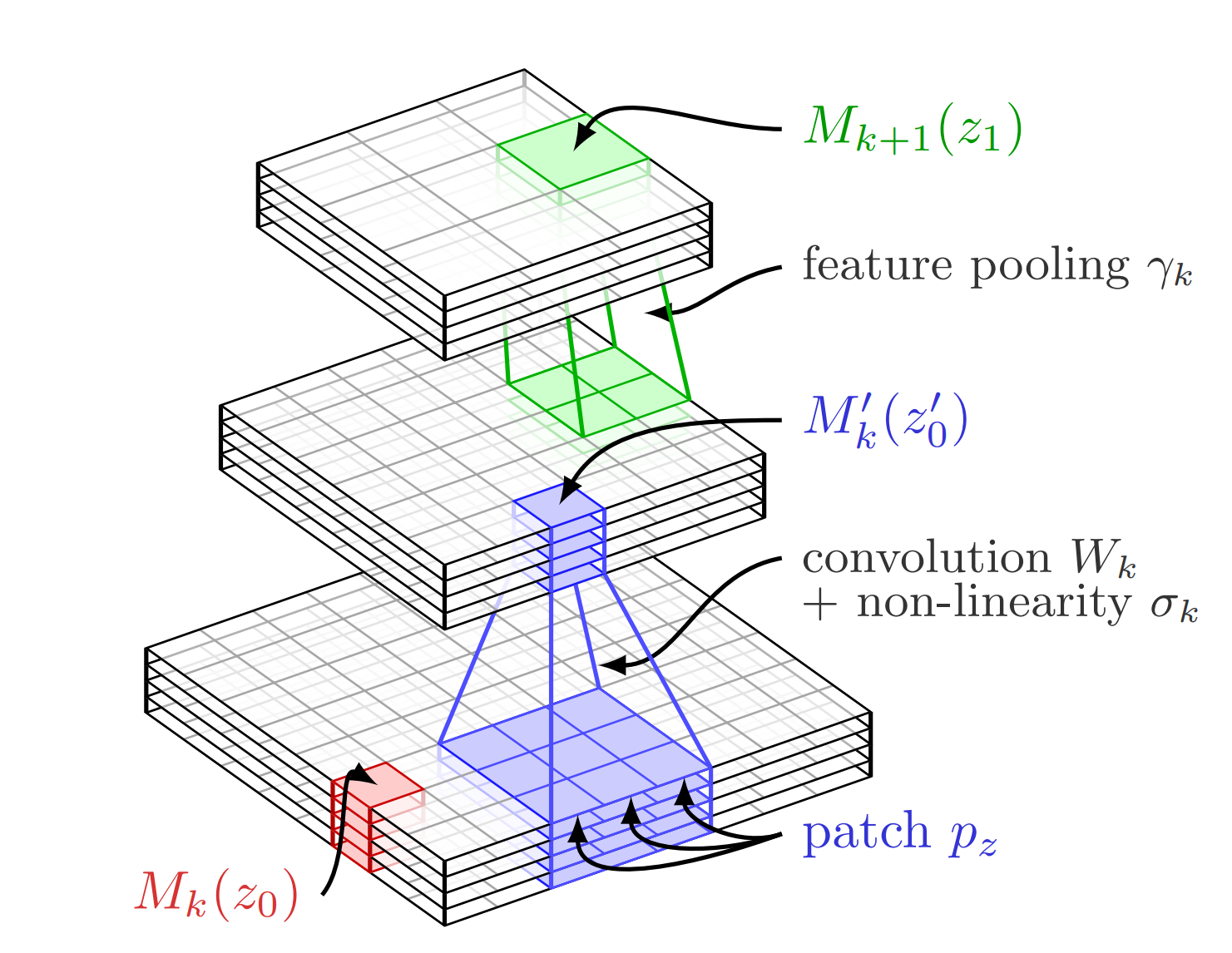
Putting everything together, a Convolutional Kernel Layer can be built in three steps.
- Extract patches \(\mathbf{x}\) from the image \(I_0\).
Patch Extraction
def extract_2d_patches(self, x): h, w = self.filter_size batch_size, C, _, _ = x.shape unfolded_x = np.lib.stride_tricks.sliding_window_view(x, (batch_size, C, h, w)) unfolded_x = unfolded_x.reshape(-1, self.patch_dim) return unfolded_x def sample_patches(self, x_in, n_sampling_patches=1000): patches = self.extract_2d_patches(x_in) n_sampling_patches = min(patches.shape[0], n_sampling_patches) patches = patches[:n_sampling_patches] return patches - Normalize and convolve them as \(\lVert \mathbf{x} \rVert \kappa \left( \mathbf{Z}^\top \displaystyle\frac{\mathbf{x}}{||\mathbf{x}||} \right)\) and compute the approximation as \(\psi(x) = \lVert \mathbf{x} \rVert\kappa\left(\mathbf{Z}^\top \mathbf{Z}\right)^{-1/2}\kappa\left(\mathbf{Z}^\top \displaystyle\frac{\mathbf{x}}{||\mathbf{x}||}\right)\) by applying the linear transform \(\kappa\left(\mathbf{Z}^\top \mathbf{Z}\right)^{-1/2}\) at every pixel location,
Convolutional Layer
def conv_layer(self, x_in): patch_norm = np.sqrt(np.clip(conv2d_scipy(x_in**2, self.ones, bias=None, stride=1, padding=self.padding, dilation=self.dilation, groups=self.groups), a_min=EPS, a_max=None)) x_out = conv2d_scipy(x_in, self.weight, self.bias, (1,1), self.padding, self.dilation, self.groups) x_out = x_out / np.clip(patch_norm, a_min=EPS, a_max=None) x_out = patch_norm * self.kappa(x_out) return x_out def mult_layer(self, x_in, lintrans): batch_size, in_c, H, W = x_in.shape x_out = np.matmul( np.tile(lintrans, (batch_size, 1, 1)), x_in.reshape(batch_size, in_c, -1)) return x_out.reshape(batch_size, in_c, H, W) -
Apply pooling operations. Note that Gaussian linear pooling is defined as
\[\begin{equation*} \displaystyle I_1(x) = \int_{\mathbf{x}'\in\Omega_0} M_1(x') \text{e}^{-\beta\lVert \mathbf{x}-\mathbf{x}'\rVert_2^2}\text{d}\mathbf{x}' \end{equation*}\]where \(M_1\) is the “feature map” after the second point operation. That is why, we can interpret the pooling operation as a “convolution” operation.
Pooling Layer
def pool_layer(self, x_in):
      if self.subsampling <= 1:
          return x_in
      x_out = conv2d_scipy(x_in, self.pooling_filter, bias=None,
          stride=self.subsampling, padding=self.subsampling,
          groups=self.out_channels)
      return x_out
The figure below summarizes all those operations, providing an overview of a Convolutional Kernel layer.
Multi-layer CKN
The first principles presented above enable to obtain a “feature map” \(I_1 \colon \Omega_1 \to \mathbb{R}^{p_1}\) from the original image \(I_0 \colon \Omega_0 \to \mathbb{R}^{3}\). Applying the same procedure leads to another map \(I_2 \colon \Omega_2 \to \mathbb{R}^{p_2}\), and another map \(I_3 \colon \Omega_3 \to \mathbb{R}^{p_3}\), and so on and so forth. In summary, a multilayer CKN consists of stacking multiple Convolutional Kernel layers. It should be noted that similarly to the convolutional neural network (CNN), the \(I_k \in \mathbb{R}^k\) represent larger and larger image neighborhoods with \(k\) increasing, gaining more invariance thanks to the pooling layers.
CNN vs. CKN ⚔️
In this part, we recall the main differences between the vanilla convolutional neural network (CNN) and the convolutional kernel network (CKN). It should be noted that the CKN is a type of CNN where the representation learning relies on the kernel trick.
Overview
In
The similarities and differences between CKN and CNN are well illustrated in the two previous figures.
On the one hand, A CNN of \(L\) layer can be represented by its output \(f_{\text{CNN}}(\mathbf{x})\), if \(\mathbf{x}\) is the input, as
\[\begin{equation*} f_{\text{CNN}}(\mathbf{x}) = \gamma_L(\sigma_L(W_L\dots \gamma_2(\sigma_2(W_2\gamma_1(\sigma_1(W_1\mathbf{x}))\dots)), \end{equation*}\]where \((W_k)_k\) represent the convolution operations, \((\sigma_k)_k\) are pointwise non-linear functions, (e.g., ReLU), and \((\gamma_k)_k\) represent the pooling operations (see
On the other hand, A CKN of \(L\) layer can be represented by its output \(f_{\text{CKN}}(\mathbf{x})\), if \(\mathbf{x}\) is the input, as
\[\begin{equation*} f_{\text{CKN}}(\mathbf{x}) = \gamma_L(\sigma_L(W_L(P_L\dots \gamma_2(\sigma_2(W_2(P_2(\gamma_1(\sigma_1(W_1(P_1(\mathbf{x}))\dots)), \end{equation*}\]where \((P_{k})_{k}\) represent the patch extractions, \((W_{k})_{k}\) the convolution operations, \((\sigma_{k})_{k}\) the kernel operations (which allows us to learn non-linearity in the RKHS), and \((\gamma_{k})_{k}\) the pooling operations.
Getting your hands dirty 🖥️
In this section, we discuss the implementation of the CKN architecture and show how to reimplement it from scratch.
Modern Implementation
The original implementation of the CKN architecture makes use of modern deep learning frameworks such as PyTorch, TensorFlow or JAX and can be found here. We recommend using it if the performance is at stake.
Stonage ML
To better understand how things work, we decided to reimplement the CKN architecture without using modern Deep Learning frameworks. It saves you the trouble of reading hundreds of documentation pages, but in return, the computational efficiency is worse for large-scale applications. Our open-source implementation of the full CKN architecture from scratch can be found here.
Autodiff
Automatic differentiation (autodiff) is a well-known algorithm that is absolutely essential in deep learning. It allows us to update the parameters of a network, by computing the derivatives with the chain rule thanks to a computational graph. If you want to implement from scratch this algorithm, you will have to implement from scratch an efficient computational graph.
Backprop in neural networks is reverse mode auto-diff applied to a simple linear computational graph. The simplicity of the resulting algorithm somehow overshadows the power and non-triviality of applying auto-diff to complex (e.g. recursive) graphs. https://t.co/5op8P7oYrE pic.twitter.com/ETafufgGqa
— Gabriel Peyré (@gabrielpeyre) January 26, 2018
For implementation from scratch details of autodiff, see this really simple blog post from Emilio Dorigatti’s website. But let’s go back to our CKN now.
Given a training set of \(n\) images \((I_{0}^1\), \(I_{0}^2, \ldots, I_{0}^n)\), optimizing a CKN of \(L\) layers consists of jointly minimizing the following optimization problem with respect to \(\mathbf{W} \in \mathbb{R}^{p_L \times \lvert\Omega_L\rvert}\) and with respect to the set of filters \(\mathbf{Z}_1,\ldots,\mathbf{Z}_L\)
\[\begin{equation*} \min_{\begin{aligned}&\mathbf{W} \in \mathbb{R}^{p_L \times \lvert\Omega_L\rvert}\\ &\mathbf{Z}_1,\ldots,\mathbf{Z}_L\end{aligned}} \frac{1}{n} \sum_{i=1}^n \mathcal{L}( y_i, \langle \mathbf{W} , I_{L}^i \rangle ) + \frac{\lambda}{2} \lVert \mathbf{W} \rVert_{\text{F}}^2 \end{equation*}\]where \(\mathcal{L}\) is a loss function, \(\lVert \cdot \rVert_{\text{F}}\) is the Frobenius norm that extends the Euclidean norm to matrices, and, with abuse of notation, the maps \(I_{k}^i\) are seen as matrices in \(\mathbb{R}^{p_L \times \lvert\Omega_L\rvert}\).
Optimizing with respect to \(\mathbf{W}\) is straightforward with any gradient-based method.
Optimizing with respect to the \(Z_j, j \in \{1,\ldots, L\}\) is a bit more tricky, as we have to examine the quantity \(\nabla_{\mathbf{Z}_{j}} \mathcal{L} (y_i, \langle \mathbf{W} , I_{L}^i \rangle)\), for \(j \in \{1,\ldots, L\}\) to compute the derivative. Once it is done, we can just use autodiff. The formulation of the chain rule is not straightforward, please check
Convolutional operations
Little-known fact: torch.conv2D computes a cross-correlation, not a convolution (yeah, the name is confusing! ![]() ). But what is the difference? The discrete convolution operator \(\ast\) between two functions \(g\) and \(h\) is defined as
). But what is the difference? The discrete convolution operator \(\ast\) between two functions \(g\) and \(h\) is defined as
whereas the discrete cross-correlation operator \(\circledast\) is defined as
\[\begin{equation*} (g \circledast h)[n]=\sum_{m=-\infty}^{\infty} \overline{g[m]} h[n+m] \end{equation*}\]where \(\overline{g[m]}\) denotes the complex conjugate of \(g[m]\). It’s subtle, but in the case of images, cross-correlation requires one less “image flipping” than convolution because of the minus sign in \(h[n-m]\). Given the number of convolutions we’re going to calculate, if we can spare ourselves an “image flip” each time, we’ll do it! What’s more, as the filter parameters are learnable, it doesn’t matter if we choose cross-correlation rather than convolution.
That being said, let’s underline the fact that accelerating the correlation operations is crucial, as it is very much part of the framework. In fact, we use correlations for convolutional layers, but we’ve also implemented linear pooling as a correlation! These operations will be performed so frequently that, with an implementation from scratch, it is absolutely essential to parallelize the process, to make it run much faster on GPUs.
Parallelization ⛷️
We’re not allowed to use torch.nn.functional.conv2d, so to parallelize scipy.signal.correlate2d, we’re left with two solutions.
1. Use CuPy!
CuPy is an open-source library for GPU-accelerated computing with Python programming language. CuPy shares the same API set as NumPy and SciPy, allowing it to be a drop-in replacement to run NumPy/SciPy code on GPU.
On top of that, CuPy has its own implementation of scipy.signal.correlate2d here, and it performs superbly. See the code below for a comparison with the original one, and torch.nn.functional.conv2d.
Execution Time
import timeit
import numpy as np
import cupy as cp
from scipy import signal
from cupyx.scipy.signal import correlate2d as cupyx_correlate2d

# Creating a test image and kernel
image = np.random.rand(5000, 5000)
kernel = np.random.rand(10, 10)

# Correlation calculation with scipy.signal.correlate2d
start_time = timeit.default_timer()
result_scipy = signal.correlate2d(image, kernel, mode='valid')
scipy_time = timeit.default_timer() - start_time
print("Execution time with scipy.signal.correlate2d :", scipy_time)

# Correlation calculation with torch.nn.functional.conv2d
start_time = timeit.default_timer()
result_torch = torch_correlate2d(image, kernel, padding='valid')
torch_time = timeit.default_timer() - start_time
print("Execution time with torch.nn.functional.conv2d :", torch_time)

# Correlation calculation with cupyx.scipy.signal.correlate2d
image_gpu = cp.asarray(image)
kernel_gpu = cp.asarray(kernel)
start_time = timeit.default_timer()
result_cupyx = cupyx_correlate2d(image_gpu, kernel_gpu, mode='valid')
cupyx_time = timeit.default_timer() - start_time
print("Execution time with cupyx.scipy.signal.correlate2d :", cupyx_time)
Running the code above produces the following output:
scipy.signal.correlate2d : 8.6376 seconds
torch.nn.functional.conv2d : 0.1617 seconds
cupyx.scipy.signal.correlate2d : 0.0006 seconds
Note that there also exist a LAX-backend implementation of scipy.signal.correlate2d in JAX.
2. Use a Low-Level Language
You can also implement the function in a low-level language such as C or C++ for better performance, and use a high-level language like Python to call this implementation. In practice, this is what is done in PyTorch. In our work, we re-implemented the scipy.signal.correlate2d using Nvidia CUDA. We provide below the corresponding implementation.
CUDA Implementation
extern "C" {
    __global__ void correlate2d_gpu_kernel(
        float* result,
        float* image,
        float* kernel,
        int image_width,
        int image_height,
        int kernel_width,
        int kernel_height) {
        int i = blockIdx.x * blockDim.x + threadIdx.x;
        int j = blockIdx.y * blockDim.y + threadIdx.y;

        if (i < image_width - kernel_width + 1 && j < image_height - kernel_height + 1) {
            float sum = 0.0f;
            for (int ki = 0; ki < kernel_width; ki++) {
                for (int kj = 0; kj < kernel_height; kj++) {
                    sum += kernel[ki * kernel_width + kj] * image[(i + ki) * image_width + (j + kj)];
                }
            }
            result[i * (image_height - kernel_height + 1) + j] = sum;
        }
    }

    void correlate2d_gpu(
        float* result,
        float* image,
        float* kernel,
        int image_width,
        int image_height,
        int kernel_width,
        int kernel_height) {
        float* d_result;
        float* d_image;
        float* d_kernel;

        cudaMalloc((void**)&d_result, (image_width - kernel_width + 1) * (image_height - kernel_height + 1) * sizeof(float));
        cudaMalloc((void**)&d_image, image_width * image_height * sizeof(float));
        cudaMalloc((void**)&d_kernel, kernel_width * kernel_height * sizeof(float));

        cudaMemcpy(d_image, image, image_width * image_height * sizeof(float), cudaMemcpyHostToDevice);
        cudaMemcpy(d_kernel, kernel, kernel_width * kernel_height * sizeof(float), cudaMemcpyHostToDevice);

        dim3 blockSize(16, 16);
        dim3 gridSize((image_width - kernel_width + 1 + blockSize.x - 1) / blockSize.x, (image_height - kernel_height + 1 + blockSize.y - 1) / blockSize.y);

        correlate2d_gpu_kernel<<<gridSize, blockSize>>>(d_result, d_image, d_kernel, image_width, image_height, kernel_width, kernel_height);

        cudaMemcpy(result, d_result, (image_width - kernel_width + 1) * (image_height - kernel_height + 1) * sizeof(float), cudaMemcpyDeviceToHost);

        cudaFree(d_result);
        cudaFree(d_image);
        cudaFree(d_kernel);
    }
}
And the Cython which has the benefit of being fast while preserving a significant part of the Python syntax.
Cython Implementation
# cython: language_level=3
import numpy as np
cimport numpy as np
from libc.math cimport floor

def correlate2d_cython(np.ndarray[np.float64_t, ndim=2] image, np.ndarray[np.float64_t, ndim=2] kernel):
    cdef int image_height = image.shape[0]
    cdef int image_width = image.shape[1]
    cdef int kernel_height = kernel.shape[0]
    cdef int kernel_width = kernel.shape[1]
    cdef int result_height = image_height - kernel_height + 1
    cdef int result_width = image_width - kernel_width + 1
    cdef np.ndarray[np.float64_t, ndim=2] result = np.zeros((result_height, result_width), dtype=np.float64)
    cdef int i, j, m, n

    for i in range(result_height):
        for j in range(result_width):
            for m in range(kernel_height):
                for n in range(kernel_width):
                    result[i, j] += image[i + m, j + n] * kernel[m, n]

    return result
Conclusion
In this blogpost, we focused on the architecture and implementation of the Convolutional Kernel Network, which plays with convolutional representations in RKHS. We take a look at its architecture and try to implement it from scratch, to better understand its ins and outs.
To find out more, the reader is invited to read Alberto Bietti’s excellent Ph.D. thesis on the subject
Acknowledgments 🙏🏾
We would especially like to thank Prof. Julien Mairal for taking the time to proofread this blog post. This is all the more important to us as he is the author of the CKN paper. We are very grateful to the professors of the Kernel Methods course of the MVA Master: Prof. Julien Mairal, Prof. Michel Arbel, Prof. Jean-Philippe Vert and Prof. Alessandro Rudi for introducing us to this field.
For any further questions, please feel free to leave a comment or contact us by mail!